An introduction to NEMF¶

The network-based ecosystem modelling framework (NEMF) is a python software tool to model ecosystems. From a modelling perspective, it consists of three conceptual parts:

Network-based model description: Each model is described by a network. A network consists of two components. Nodes, which describe ecosystem compartments, and edges, which link two compartments together through some interaction.
Forward modelling: A model is defined by a set of differential equations implicitly defined by the network structure. Theses differential equations can be solved numerically for a certain initial state. Hence, providing forecasts for how the model behave over time.
Inverse modelling: Fitting of model forecast to to observational or other reference data, by varying model parameters.

It aims to keep the configuration complexity minimal for the user such that it can be quickly learned and applied for i.e. rapid prototyping of model ideas. To keep configuration and computational complexity low it can only applied to non-spatially-resolved, also known as box-models.

Network and Forward¶

We will now go over the the first two parts of the model with the help of a simple NPZD type model. NPZD stands for the Nutrient- Phytoplankton- Zooplanktion-Detritus model, which is a simple well studied marine ecosystem model. The details of it are not important here, as it is solely used as placeholder for any sort of ecosystem model.

To calculate the forecast of a model we run the following few lines of code:

import nemf
model_path = 'emplary_npzd_model.yml'
model = nemf.load_model(model_path)
nemf.interaction_graph(model)
output_forward = nemf.forward_model(model)
nemf.output_summary(output_forward)

Let’s go through the lines one by one to see what happened:

First we imported the nemf python library.
```
import nemf
```
This tells python that we want to us this library and because not stated otherwise that we will address it as nemf
We tell the nemf library which model we want to use.
```
model_path = 'exemplary_npzd_model.yml'
model = nemf.load_model(model_path)
```
Models are typically defined in an extra file. This file contains the description of the model in a humon-readable standard called YAML. Hence, the file extension .yml More on the yml standard and how it is used to define models can be found here.
We visualize the network defined in the model configuration by
```
nemf.interaction_graph(model)
```
which returns the following plot:

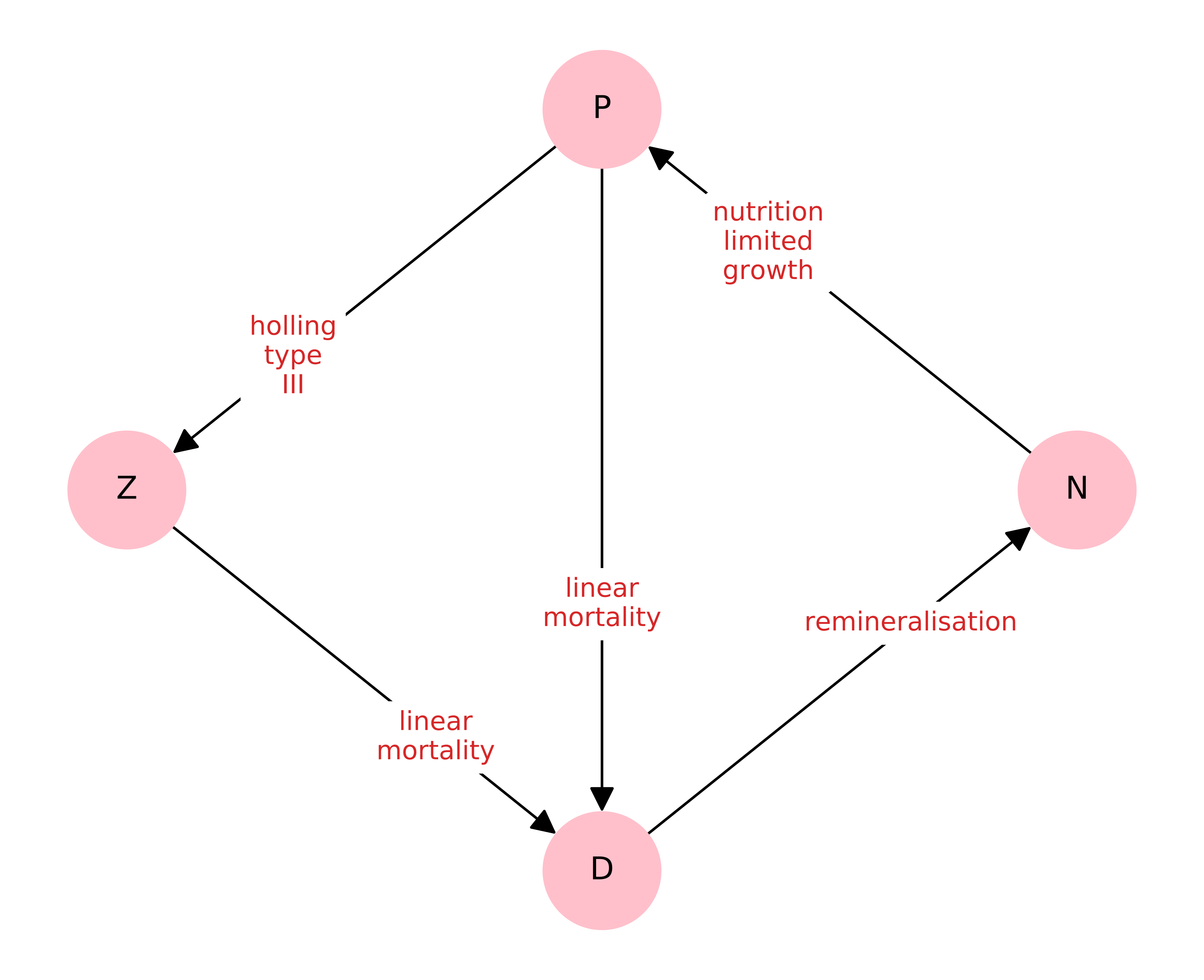
NEMF offers the option to draw the network defined in the model configuration. This is helps to catch errors that might have happened during the configuration and gives a nice overview over the model. Each node represents a compartment in the model, i.e. a population or a chemical quantity. The arrows between them show what flows from one compartment to another while the label on the arrow describes how it does that.
We solve the differential equations underlying the model numerically with:
```
output_forward = nemf.forward_model(model)
```
The network implicitly defines a set of differential equation that couples the compartments to each other, through the interactions between them. The framework solves these differential equations to give a forecast how the model is expected to evolve over time. This is often also called ‘time evolution’.
The result of the time evolution are visualized by calling
```
nemf.output_summary(output_forward)
```
which generates the following plot:

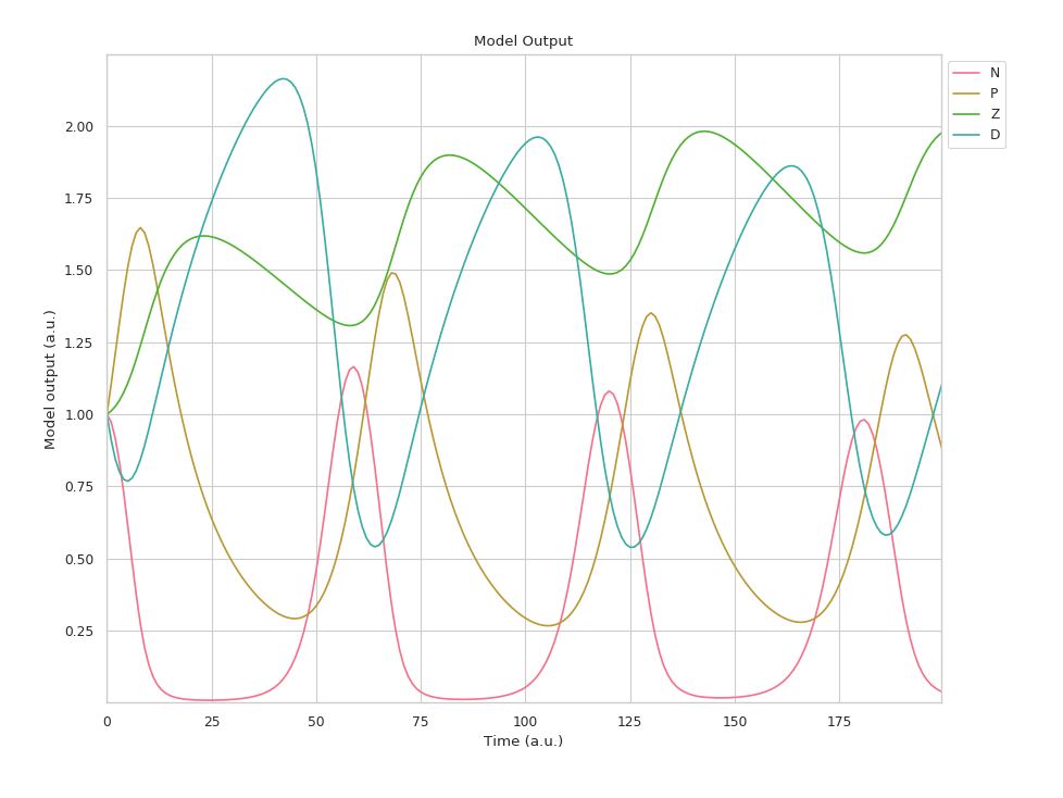
Each line represents one compartment and how its associated quantity (i.e. a population size) changes over time.

Model description via YAML configuration¶

In the example above, we assumed that a model (‘exemplary_npzd_model’) has already been defined. If we want to construct a new model, we need to write our own configuration file.

There are three major parts of the configuration file:

Compartments contain a list of all model compartments, like species population pools or nutrition pools.
Interactions contains a list of all interactions between compartments, like what eats what and what happens when it dies
Configuration contains a list of technical details that decide the framework behavior during the forecast and fitting.

The configuration file is written in the YAML standard.

It consists of what is called key-value pairs. Each key is associated with a value. These values can also be lists which are indicated by leading “-“, like bullet points. You can find details about the YAML standard on http://yaml.org/. Note that the YAML website is itself perfectly valid yaml.

A simple example for the compartment section looks like this:

compartment:      # header of the compartment section
  A:              # name of compartment
    value: 1.0    # initial value of the compartment
  B:
    value: 2.0
  ..
  ..

Interactions are defined similarly:

A:B:              # flow from B to A (predator:prey)
- fkt: grazing    # type of interaction
- parameters:     # parameters used for the interaction
  - 1             # i.e. hunting rate
  - 2             #      food processing time
B:A
- fkt: natural mortality
- parameters:
  - 0.01          # natural mortality rate

A description of how this works in detail can be found in the YAML section of the manual.

Inverse modelling¶

So far, we covered the first two aspect; the network-based approach and the forward modelling. We can also fit unknown, or imprecisely known parameters such that the forecast resembles a provided data set as closely as possible.

We can achieve this with the inverse_model method.

import nemf
model_path = 'path/to/the/yaml/file/presented/above/example.yml'
reference_data_path = 'path/to/the/data/file/representing/the/model_ref.csv'
model = nemf.load_model(model_path,reference_data_path)
output_inverse = nemf.inverse_model(model)
nemf.output_summary(output_inverse)

Most of this code is the same as previously shown. The are only two new lines. The first binds the path of the reference data file:

reference_data_path = 'path/to/the/data/file/representing/the/model_ref.csv'

This is path is then used when loading the model:

model = nemf.load_model(model_path,reference_data_path)

Hence, making both the model description as well as the reference data available to the framework.

The second new line is:

output_inverse = nemf.inverse_model(model)

Instead of calculating the forecast once as previously shown, the inverse_model now calculates it for different sets of parameters in such a way that we find the best solution quickly.

However, for this to work we provided some additional information. There are two things we need to provide:

Reference data (i.e observational data)
Optimized parameters

The reference data is expected do be in a separate file. Details about its format and how it can be imported can be found in the reference data section of the manual.

The parameters that shall be optimized are selected in the YAML configuration file by adding the ‘optimise’ key and providing its upper and lower bounds in which the method tries to find the best solution.

compartment:      # header of the compartment section
  A:              # name of compartment
    value: 1.0    # initial value of the compartment
    optimise:
      lower: 0    # lower and
      upper: 2    # upper bound during the fitting process

The reference data can either be passed directly when loading the model or alternatively be set in the yaml file as well.

Detail on the configuration of the YAML file can be found in the yaml section of the manual.

The results are then visualized with:

nemf.output_summary(output_inverse)

Which creates the following figure:

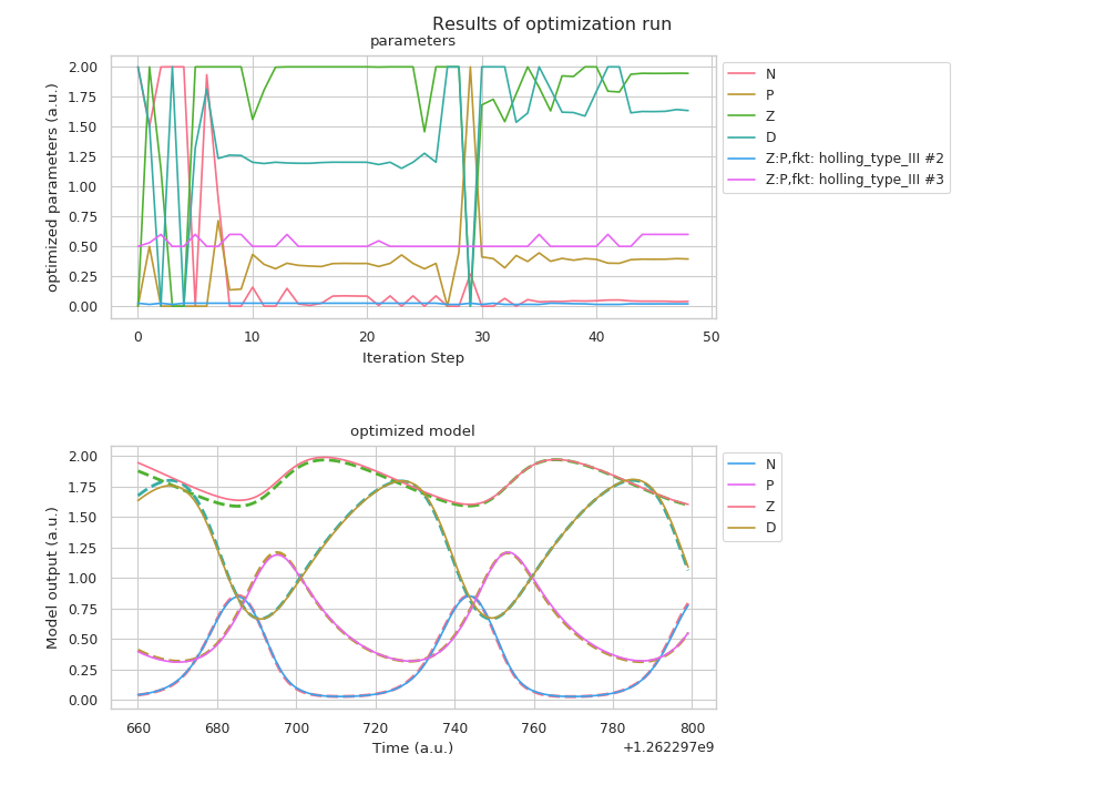
Visualization of the results of the model fit. The upper figure shows the tested parameter during the fitting process, while the lower figure shows the “optimally” fitted model.

Next steps¶

You have a few options for where to go next. You might first want to learn how to install namf on your machine. Once that’s done, you can browse the examples to get a broader sense for what kind problems nemf is designed for. You can read through the manual for a deeper discussion of the different parts of the library and how they are designed. If you want to know specifics of the nemf functions implementations, you could check out the API reference, which documents each function and its parameters.